Ik heb deze introductie ooit in het Engels opgesteld. Ik denk niet dat er ooit een vertaling komt. Als je geen Engels verstaat en toch geïnteresseeerd bent, wil ik dit gerust bij pot en pint allemaal uit de doeken doen.

Linear Algebra

Basically, linear algebra is about solving equations. An example:

(1)

The solution of (1) is of course . We can make this harder by adding an unknown:

(2)

Subtracting the first equation from the second tells us that . Then from either of the equations we learn that also . This is still rather easy, but suppose we have a lot of unknowns and a lot of equations:

(3)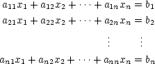

The techniques used will be very much the same as the ones to solve (2): subtracting equations to simplify things. As mathematicians are mostly lazy people, the standard notation is shortened. We start by writing (3) as

(4)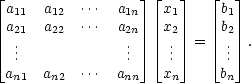

So this is exactly the same as (3), we only sorted out the mess a little. Then we can write one symbol for a whole block:

(5)

This is much more convenient to speak about. So now we have a vector of unknowns, and the known information is the matrix (this name has nothing to do with the movie and is already in use for centuries) and the right hand side . The operations to solve the system (5) (or if you prefer, the system (3)) are only applied to and , the unknowns never change during computation (otherwise we wouldn’t compute them, of course!).

Now suppose we have a matrix , a number and a vector such that

(6)

In this case we call an eigenvalue of the matrix and an eigenvector. In a lot of scientific applications it is important to be able to compute the eigenvalues of a matrix. Unfortunately, it is not possible to compute them exactly (theoretically!), so we can only approximate them.

Numerical computations

In doing computations on a computer, one should be very careful. The computer is only able to store a finite number of numbers. Since there are a lot more numbers in “real life” (funny a mathematician uses this term :), the number stored by the computer is not always the number you put in there! However, it is a good approximation: on most machines the error will be smaller then 10^-16, which is very small. The problem arises if you make a lot of computations: then every time you take in a small error, and if you’re not careful, at the end of the big computation you don’t have any accuracy left. So the main issue of Numerical Linear Algebra is to devise methods to solve systems of equations and compute eigenvalues, in such a way that the roundoff error stays small.

Convergence of algorithms

Well, an algorithm is just a solution method. A number of rules that take you from your data to the solution. Something that is easily performed by a computer. Arnoldi, Lanczos and IAP are just specific examples of eigenvalue algorithms.

One way to try to control the roundoff error is making iterative algorithms. One step of an iterative algorithm can be described as follows: you take an approximate solution, and create a better one. So at the start of your algorithm you provide an initial guess (which can be far off), and then in each step you move closer and closer to the real solution. Then you just have to figure out when to stop.

The convergence of an iterative algorithm is just the fashion in which the approximate solutions go to the real solution. This can be fast/slow, monotonic/erratic, …

Potential theory

Now for something completely different. The techniques I use to examine the convergence of iterative algorithms are based on some complex analysis. I will need the concept of a measure. A measure is a function that assigns a number to every set. For example: the number of elements inside the set (but there are far more measures). There are some conditions a set function has to satisfy before you can call it a measure, but I won’t go into detail.

Once you have a measure, say , you can construct an integral. An integral is a functional (some kind of function) that assigns a number to each function. This is done by first looking at the “basis functions” that take the value 1 on the set and 0 outside that set. Then we define

(7)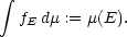

We can do this for every set. Then this definition can be extended to all functions, by taking an arbitrary function and looking at it as a combination of basis functions.

Now we have all the ingredients to define the logarithmic potential , which is a function of the variable , connected with the measure , and the logaritmic energy , which is a number (so is also a functional).

(8)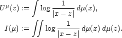

Here we use the notation in the integral to make clear to which variable we integrate.

Recapitulating

So I presented some concepts of two fields (in a simplified way): numerical linear algebra and potential theory. It is not simple to explain their connection, but for the insiders: this is accomplished by a polynomial minimization problem. Perhaps I will include a section on that later on, but for now, this has to do.